Task 3: Electromagnetic induction and the Earth’s conductivity
In this task, we will apply a novel processing of Swarm magnetic field measurements to unravel the electrical conductivity of the lower mantle, using the electromagnetic induction process driven by 1) large geomagnetic storms in the magnetosphere, and 2) secular variation of the core field.
WINTERC-e is an upper mantle (down to 400 km depth) electrical conductivity model produced in the context of ESA’s Support to Science Element project 3D Earth (Martinec et al., 2021). WINTERC-e is based on the thermal and compositional fields from WINTERC-G (constrained by surface wave tomography + satellite gravity + SHF and isostasy) and laboratory studies on the conductivity of the main upper mantle minerals including the effects of water and melt.
Despite being totally independent from magnetic data, WINTERC-e reproduces well the first order tidal magnetic field M2 inferred from Swarm data. Here we will test the sensitivity of MMC data to variations in the volatile content (water, melt) using WINTERC-e as a test bed.
Workpackages Task 3
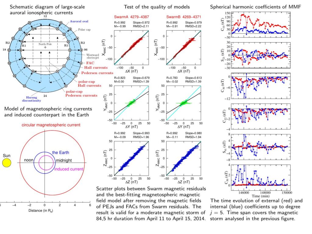
To run the sensitivity analysis, we will use the forward and inverse solver (ELMGIV_FWD, ELMGIV_INV) for electromagnetic induction (EMI) in a 3D Earth (Velímský and Martinec, 2005; Velímský 2013). The solver runs computations in time domain which is consistent with a transient time behaviour of Swarm magnetic field during large magnetic storms. The specification of the electrical conductivity of the mantle and the inducing (external) magnetic
field are required as the input data for the forward EMI code. We will start from the existing 1-D and 3-D conductivity models derived from MMA to establish the sensitivity of MMC to conductivity variations in the ULM. A misfit between the internal part of MMC, and the prediction of the numerical simulations will be complemented by calculations of its first and second derivatives with respect to conductivity parameters, using the adjoint method (Maksimov and Velímský, 2017).
We will consider the magnetic field at the CMB as provided by the recent core dynamo models (e.g. Aubert et al., 2017, Davies et al., 2022). Having specified the tangential components of SV on the CMB, we will run the forward EMI solver ELMGIV_FWD, as described in WP 3100. In contrast to the previous case, we will modify it in such a way, that the boundary conditions on the lower boundary (i.e., CMB) are specified. We will use different types of 1-D and 3-D lower-mantle conductivity models, partly obtained by analysis of induction responses at very long periods (Constable, 2022), and partly based on the temperature and composition distributions derived from body wave and normal mode seismic tomography, and satellite gravity data modelling together with laboratory conductivity estimates for lower mantle minerals, The sensitivity analysis will vary the amplitudes and distributions of LM conductivities and continue the magnetic field upward from the core to the Earth surface. Comparing the modelled and observed SV on the Earth surface will provide the information on the sensitivity of surface SV on LM conductivities.